Word Clouds from Adjusted Counts
By: Jeff Clark Date: Tue, 07 Jul 2009
When trying to understand something it is often very useful to compare and contrast the data of interest with some related data. This can serve to emphasize the unique characteristics of the data you are studying. Another way of thinking about it is that you are filtering out the background noise in order to clarify the signal.
I mentioned in the recent post Shaped Word Cloud: Canada that I had adjusted the word counts according to how frequently they occurred in a baseline dataset. In this post I give a graphic example of the effects of this type of adjustment.
The data used is a collection of 16,504 tweets gathered during the month of June, 2009 and containing the word 'starbucks' . They are every 10th tweet of the full 165,040 that I collected during this time period. I also discarded the tweets that were obviously non-English. The words 'starbucks' , 'coffee' , and any twitter ID were not used in the analysis.
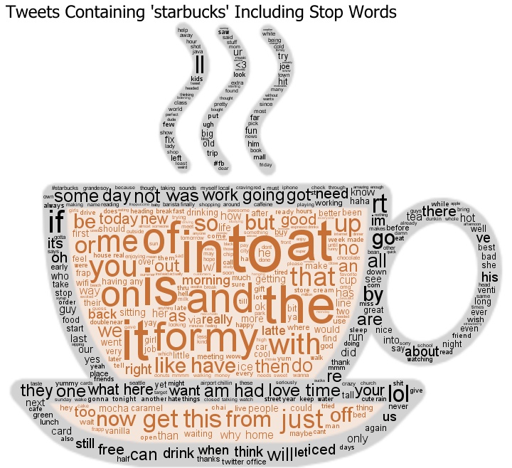
The following word cloud was constructed from the word frequencies found. It includes stop words and the cloud shows that 'in' , 'to' , 'at', 'is' and many other small words are frequently used in the text. The problem is that this is true for any sizable amount of English text and so this word cloud doesn't illustrate any real useful information specific to 'starbucks'. For this reason, stop words are almost always excluded from word clouds.
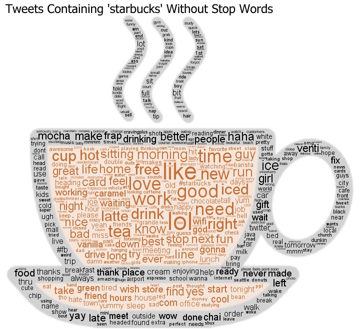
This next cloud was generated from the same data and the only change was that stop words were excluded. Now we can start to see some interesting emotion-laden words like 'love' , 'good' , 'work' , 'like' as well as some that are obviously characteristic of the search term like 'hot' , 'cup', 'mocha', 'frap', and 'drinking'.
To reveal more detail specific to 'starbucks' I have adjusted the word counts in this final cloud based on how frequently the words occurred in a baseline data set. The baseline I used here was a collection of tweets containing the word 'coffee' taken over the same time period as the original starbucks tweets. I won't describe the math in detail but, basically, I boosted the counts for words by a factor that is a function of the word frequency rate in the two data sets. If a word is used much more frequently in the starbucks data than the coffee data then it's count is elevated so that it becomes more prominent in the cloud.
This word cloud is much more revealing of those things discussed in tweets together with 'starbucks'. Some of the large terms include, '#starbucks', several variations on 'frap', 'ruling', 'fructose', 'lemonade', 'venti', 'card', and 'sponsorship'.

By choosing different baseline datasets it is possible to accentuate different perspectives of the original data. For example, breaking down a collection of tweets by geographic origin and contrasting the data using this technique would let you uncover geographic patterns. What are people saying about Starbucks in San Francisco that is different from what they say in New York , or London ? If you break up the tweet collection by time you can answer questions like: What are people saying about Starbucks at lunchtime versus in the morning ? Or, What are they saying on Tuesdays versus Saturdays ?
I believe this technique may prove very useful in revealing information from large amounts of text.